
Notice
Recent Posts
Recent Comments
Link
| 일 | 월 | 화 | 수 | 목 | 금 | 토 |
|---|---|---|---|---|---|---|
| 1 | ||||||
| 2 | 3 | 4 | 5 | 6 | 7 | 8 |
| 9 | 10 | 11 | 12 | 13 | 14 | 15 |
| 16 | 17 | 18 | 19 | 20 | 21 | 22 |
| 23 | 24 | 25 | 26 | 27 | 28 |
Tags
- 파트5
- 빅데이터분석기사
- backtest
- 실기
- 파이썬
- 파이썬 주식
- Programmers
- SQL
- 백테스트
- 토익스피킹
- TimeSeries
- randomforest
- hackerrank
- 변동성돌파전략
- Crawling
- sarima
- 데이터분석전문가
- GridSearchCV
- docker
- 프로그래머스
- 데이터분석
- Quant
- 비트코인
- 볼린저밴드
- ADP
- 코딩테스트
- 주식
- lstm
- Python
- PolynomialFeatures
Archives
- Today
- Total
데이터 공부를 기록하는 공간
볼린저밴드-추세추종 본문
""" 시간대별 데이터 불러오기 """
import pandas as pd
import numpy as np
import matplotlib.pyplot as plt
import pyupbit

df = pyupbit.get_ohlcv("KRW-BTC", interval = "minute60", count=2000)
print(df)
■ 볼린저밴드- 추세추종
df = data.copy()
df['MA20'] = df['close'].rolling(window=20).mean()
df['stddev'] = df['close'].rolling(window=20).std()
df['upper'] = df['MA20'] + df['stddev']*2
df['lower'] = df['MA20'] - df['stddev']*2
### PB : %b (종가 - 하단밴드) / (상단밴드 - 하단밴드) ###
df['PB'] = (df['close'] - df['lower']) / (df['upper'] - df['lower'])
### 밴드폭 (상단밴드 - 하단밴드) / 중간밴드
df['bandwidth'] = (df['upper'] - df['lower']) / df['MA20'] * 100
### 중심가격
df['TP'] = (df['high'] + df['low'] + df['close']) / 3
### 긍정적 현금 흐름 : 중심가격이 전일보다 상승한 날들의 현금 흐름의 합
df['PMF'] = 0
### 부정적 현금 흐름 : 중심가격이 전일보다 하락한 날들의 현금 흐름의 합
df['NMF'] = 0
for i in range(len(df.close)-1):
    if df.TP.values[i] < df.TP.values[i+1]: # TP값이 전날보다 증가한다면,
        df.PMF.values[i+1] = df.TP.values[i+1] * df.volume.values[i+1]
        df.NMF.values[i+1] = 0
    else:
        df.PMF.values[i+1] = 0
        df.NMF.values[i+1] = df.TP.values[i+1] * df.volume.values[i+1]
### 현금 흐름 비율 : Money Flow Ratio
df['MFR'] = df.PMF.rolling(window=10).sum() / df.NMF.rolling(window=10).sum()
### 현금 흐름 지표 : Money Flow Index = 100 - ( 100 ÷ (1+MFR) )
df['MFI'] = 100 - 100 / (1+df['MFR'])
df = df.dropna()
df = df[:500]
fig, (ax1, ax2) = plt.subplots(nrows=2, figsize=(9,8))
ax1.plot(df.index, df['close'], color='#0000ff', label='close')
ax1.plot(df.index, df['upper'], 'r--', label='upper band')
ax1.plot(df.index, df['lower'], 'c--', label='lower band')
ax1.plot(df.index, df['MA20'], 'k--', label='MA20')
ax1.fill_between(df.index, df['upper'], df['lower'], color='0.9')
for i in range(len(df.close)):
if df.PB.values[i] > 0.8 and df.MFI.values[i] > 80:
ax1.plot(df.index.values[i], df.close.values[i], 'r^')
elif df.PB.values[i] < 0.2 and df.MFI.values[i] < 20:
ax1.plot(df.index.values[i], df.close.values[i], 'bv')
ax1.legend(loc='best')
ax2.plot(df.index, df['PB']*100, 'b', label= '%B x 100')
ax2.plot(df.index, df['MFI'], 'g--', label='MFI(10 day)')
ax2.set_yticks([-20, 0, 20, 40, 60, 80, 100, 120])
for i in range(len(df.close)):
if df.PB.values[i] > 0.8 and df.MFI.values[i] > 80:
ax2.plot(df.index.values[i], 0, 'r^')
elif df.PB.values[i] < 0.2 and df.MFI.values[i] < 20:
ax2.plot(df.index.values[i], 0, 'bv')
#ax2.grid(True)
ax2.legend(loc='best')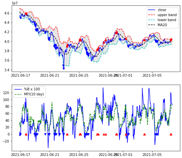
df['return'] = np.log(df['close']/df['close'].shift(1)) # 로그수익률
## df.PB.values[i] > 0.8 and df.MFI.values[i] > 80:
cond_buy = (df['PB'] > 0.8) & (df['MFI'] > 80)
df.loc[cond_buy, 'position'] = 1
## df.PB.values[i] < 0.2 and df.MFI.values[i] < 20:
cond_sell = (df['PB'] < 0.2) & (df['MFI'] < 20)
df.loc[cond_sell, 'position'] = 0
df['position'] = df['position'].fillna(method = "ffill")
df['strategy'] = df['position']*df['return']
df[['return','strategy']].sum().apply(np.exp)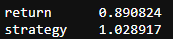
df[['return','strategy']].cumsum().apply(np.exp).plot(figsize=(9,6))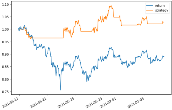
한번에 그리기
df = data.copy()
df['MA20'] = df['close'].rolling(window=20).mean()
df['stddev'] = df['close'].rolling(window=20).std()
df['upper'] = df['MA20'] + df['stddev']*2
df['lower'] = df['MA20'] - df['stddev']*2
### PB : %b (종가 - 하단밴드) / (상단밴드 - 하단밴드) ###
df['PB'] = (df['close'] - df['lower']) / (df['upper'] - df['lower'])
### 밴드폭 (상단밴드 - 하단밴드) / 중간밴드
df['bandwidth'] = (df['upper'] - df['lower']) / df['MA20'] * 100
### 중심가격
df['TP'] = (df['high'] + df['low'] + df['close']) / 3
### 긍정적 현금 흐름 : 중심가격이 전일보다 상승한 날들의 현금 흐름의 합
df['PMF'] = 0
### 부정적 현금 흐름 : 중심가격이 전일보다 하락한 날들의 현금 흐름의 합
df['NMF'] = 0
for i in range(len(df.close)-1):
    if df.TP.values[i] < df.TP.values[i+1]: # TP값이 전날보다 증가한다면,
        df.PMF.values[i+1] = df.TP.values[i+1] * df.volume.values[i+1]
        df.NMF.values[i+1] = 0
    else:
        df.PMF.values[i+1] = 0
        df.NMF.values[i+1] = df.TP.values[i+1] * df.volume.values[i+1]
### 현금 흐름 비율 : Money Flow Ratio
df['MFR'] = df.PMF.rolling(window=10).sum() / df.NMF.rolling(window=10).sum()
### 현금 흐름 지표 : Money Flow Index = 100 - ( 100 ÷ (1+MFR) )
df['MFI'] = 100 - 100 / (1+df['MFR'])
df['return'] = np.log(df['close']/df['close'].shift(1)) # 로그수익률
## df.PB.values[i] > 0.8 and df.MFI.values[i] > 80:
cond_buy = (df['PB'] > 0.8) & (df['MFI'] > 80)
df.loc[cond_buy, 'position'] = 1
## df.PB.values[i] < 0.2 and df.MFI.values[i] < 20:
cond_sell = (df['PB'] < 0.2) & (df['MFI'] < 20)
df.loc[cond_sell, 'position'] = 0
df['position'] = df['position'].fillna(method = "ffill")
df['strategy'] = df['position'] * df['return']

df = df.dropna()
df = df[:500]
print("backtest results : ")
df[['return','strategy']].sum().apply(np.exp)


fig, (ax1, ax2, ax3) = plt.subplots(nrows=3, figsize=(9,8))
ax1.plot(df.index, df['close'], color='#0000ff', label='close')
ax1.plot(df.index, df['upper'], 'r--', label='upper band')
ax1.plot(df.index, df['lower'], 'c--', label='lower band')
ax1.plot(df.index, df['MA20'], 'k--', label='MA20')
ax1.fill_between(df.index, df['upper'], df['lower'], color='0.9')
for i in range(len(df.close)):
    if df.PB.values[i] > 0.8 and df.MFI.values[i] > 80:
        ax1.plot(df.index.values[i], df.close.values[i], 'r^')
    elif df.PB.values[i] < 0.2 and df.MFI.values[i] < 20:
        ax1.plot(df.index.values[i], df.close.values[i], 'bv')
ax1.legend(loc='best')
ax2.plot(df.index, df['PB']*100, 'b', label= '%B x 100')
ax2.plot(df.index, df['MFI'], 'g--', label='MFI(10 day)')
ax2.set_yticks([-20, 0, 20, 40, 60, 80, 100, 120])
for i in range(len(df.close)):
    if df.PB.values[i] > 0.8 and df.MFI.values[i] > 80:
        ax2.plot(df.index.values[i], 0, 'r^')
    elif df.PB.values[i] < 0.2 and df.MFI.values[i] < 20:
        ax2.plot(df.index.values[i], 0, 'gv')
#ax2.grid(True)
ax2.legend(loc='best')

df[['return','strategy']].cumsum().apply(np.exp).plot(ax=ax3)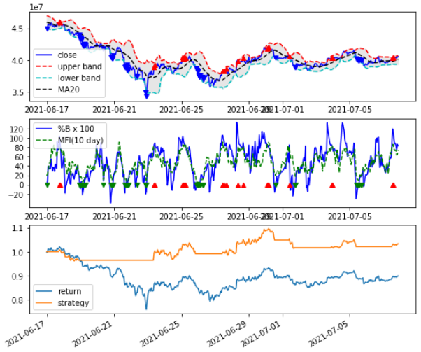
■ 함수를 활용해서 하이퍼파라미터 최적화하기 1
""" 시간대별 데이터 불러오기 """
import pandas as pd
import numpy as np
import matplotlib.pyplot as plt
import pyupbit

df = pyupbit.get_ohlcv("KRW-BTC", interval = "minute60", count=5000)
print(df)
data=df.copy()
# window_b : 볼린저밴드 윈도우
# window_f : 현금흐름지표 윈도우
# buy_pb : 매수조건 퍼센트볼린저 하한
# buy_mfi : 매수조건 현금흐름지표 하한
# sell_pb : 매도조건 퍼센트볼린저 상한
# sell_mfi : 매도조건 현금흐름지표 상한
# 0 < pb < 1
# 0 < mfi < 100
def 볼린저밴드_추세추종(data=data, window_b = 20, window_f=10, buy_pb = 0.8, buy_mfi = 80, sell_pb = 0.2, sell_mfi=20, chart=False):
df = data.copy()
df['MA20'] = df['close'].rolling(window=window_b).mean()
df['stddev'] = df['close'].rolling(window=window_b).std()
df['upper'] = df['MA20'] + df['stddev']*2
df['lower'] = df['MA20'] - df['stddev']*2
### PB : %b (종가 - 하단밴드) / (상단밴드 - 하단밴드) ###
df['PB'] = (df['close'] - df['lower']) / (df['upper'] - df['lower'])
### 밴드폭 (상단밴드 - 하단밴드) / 중간밴드
df['bandwidth'] = (df['upper'] - df['lower']) / df['MA20'] * 100
### 중심가격
df['TP'] = (df['high'] + df['low'] + df['close']) / 3
### 긍정적 현금 흐름 : 중심가격이 전일보다 상승한 날들의 현금 흐름의 합
df['PMF'] = 0
### 부정적 현금 흐름 : 중심가격이 전일보다 하락한 날들의 현금 흐름의 합
df['NMF'] = 0
for i in range(len(df.close)-1):
if df.TP.values[i] < df.TP.values[i+1]: # TP값이 전날보다 증가한다면,
df.PMF.values[i+1] = df.TP.values[i+1] * df.volume.values[i+1]
df.NMF.values[i+1] = 0
else:
df.PMF.values[i+1] = 0
df.NMF.values[i+1] = df.TP.values[i+1] * df.volume.values[i+1]
### 현금 흐름 비율 : Money Flow Ratio
df['MFR'] = df.PMF.rolling(window=window_f).sum() / df.NMF.rolling(window=window_f).sum()
### 현금 흐름 지표 : Money Flow Index = 100 - ( 100 ÷ (1+MFR) )
df['MFI'] = 100 - 100 / (1+df['MFR'])
df['return'] = np.log(df['close']/df['close'].shift(1)) # 로그수익률
## df.PB.values[i] > 0.8 and df.MFI.values[i] > 80:
cond_buy = (df['PB'] > buy_pb) & (df['MFI'] > buy_mfi)
df.loc[cond_buy, 'position'] = 1
## df.PB.values[i] < 0.2 and df.MFI.values[i] < 20:
cond_sell = (df['PB'] < sell_pb) & (df['MFI'] < sell_mfi)
df.loc[cond_sell, 'position'] = 0
df['position'] = df['position'].fillna(method = "ffill")
df['strategy'] = df['position'] * df['return']
df['cumret'] = df['strategy'].cumsum().apply(np.exp)
df['cummax'] = df['cumret'].cummax()
df = df[max(window_b, window_f):]
drawdown = df['cummax'] - df['cumret']
mdd = drawdown.max()
result = df[['return','strategy']].sum().apply(np.exp)
print("backtest results : ")
print(data.index[0] , " ~ ", data.index[-1])
print("buy : sell = " + str(df.loc[cond_buy].shape[0]) + " : " + str(df.loc[cond_sell].shape[0]))
print("return : ", np.round(result['return']*100,1),"%")
print("strategy : ", np.round(result['strategy']*100,1),"%")
print("mdd : △", np.round(mdd*100,0),"%")
if chart == True:
fig, (ax1, ax2, ax3) = plt.subplots(nrows=3, figsize=(20,8))
ax1.plot(df.index, df['close'], color='#0000ff', label='close')
ax1.plot(df.index, df['upper'], 'r--', label='upper band')
ax1.plot(df.index, df['lower'], 'c--', label='lower band')
ax1.plot(df.index, df['MA20'], 'k--', label=f'MA{window_b}')
ax1.fill_between(df.index, df['upper'], df['lower'], color='0.9')
for i in range(len(df.close)):
if df.PB.values[i] > buy_pb and df.MFI.values[i] > buy_mfi:
ax1.plot(df.index.values[i], df.close.values[i], 'r^')
elif df.PB.values[i] < sell_pb and df.MFI.values[i] < sell_mfi:
ax1.plot(df.index.values[i], df.close.values[i], 'bv')
ax1.legend(loc='best')
ax2.plot(df.index, df['PB']*100, 'b', label= '%B x 100')
ax2.plot(df.index, df['MFI'], 'g--', label=f'MFI({window_f} day)')
ax2.set_yticks([-20, 0, 20, 40, 60, 80, 100, 120])
for i in range(len(df.close)):
if df.PB.values[i] > buy_pb and df.MFI.values[i] > buy_mfi:
ax2.plot(df.index.values[i], 0, 'r^')
elif df.PB.values[i] < sell_pb and df.MFI.values[i] < sell_mfi:
ax2.plot(df.index.values[i], 0, 'gv')
#ax2.grid(True)
ax2.legend(loc='best')
df[['return','strategy']].cumsum().apply(np.exp).plot(ax=ax3)볼린저밴드_추세추종(data=data, window_b = 20, window_f=10, buy_pb = 0.8, buy_mfi = 80, sell_pb = 0.2, sell_mfi=20, chart=True)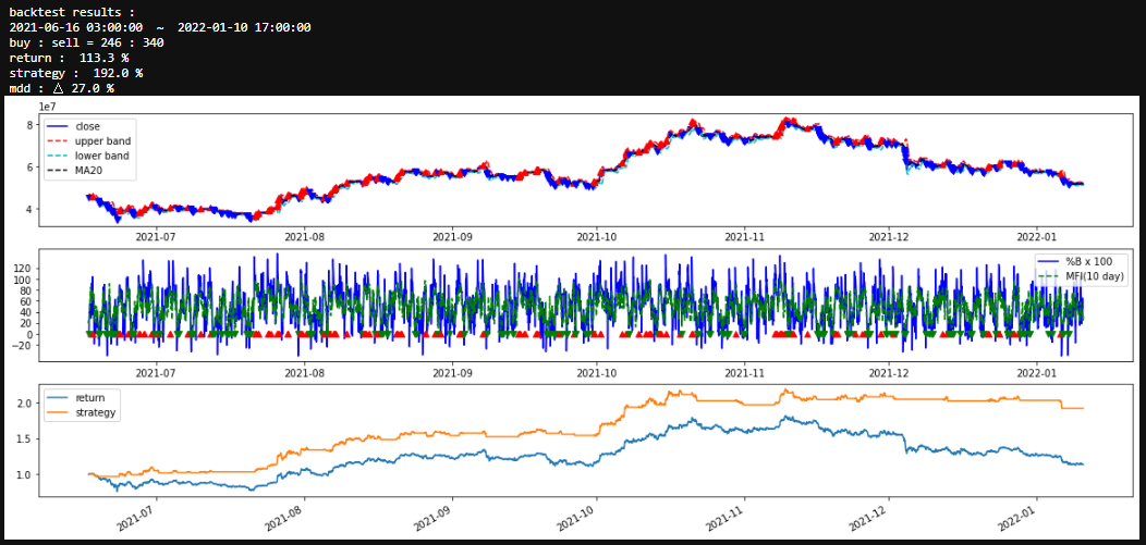
볼린저밴드_추세추종(data=data, window_b = 20, window_f=10, buy_pb = 0.9, buy_mfi = 90, sell_pb = 0.1, sell_mfi=10, chart=True)
볼린저밴드_추세추종(data=data, window_b = 20, window_f=10, buy_pb = 0.9, buy_mfi = 90, sell_pb = 0.2, sell_mfi=20, chart=True)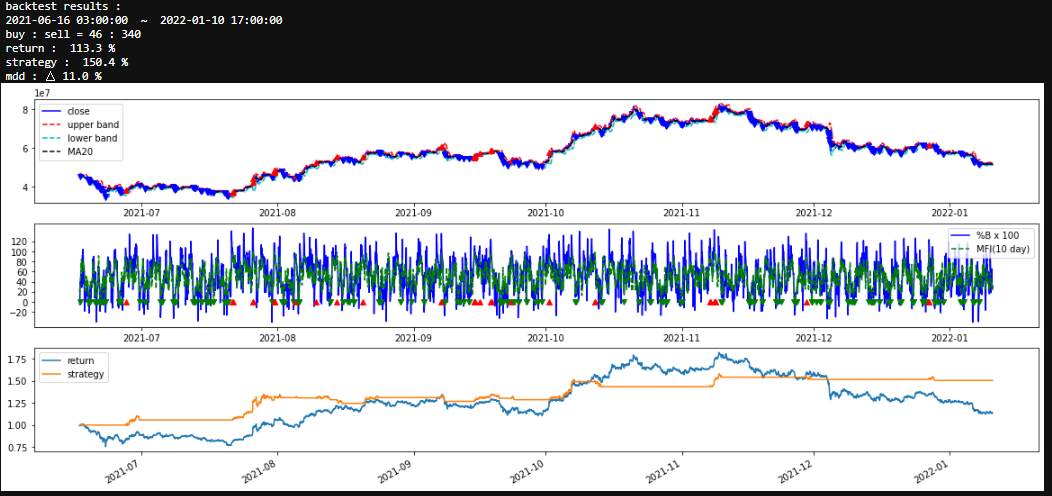
볼린저밴드_추세추종(data=data, window_b = 20, window_f=10, buy_pb = 0.8, buy_mfi = 80, sell_pb = 0.1, sell_mfi=10, chart=True)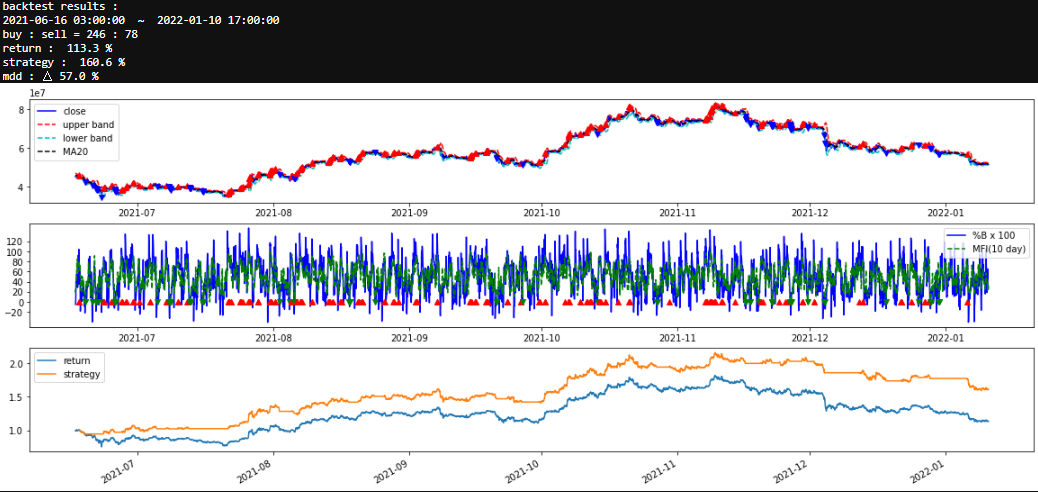
▶ buy_pb = 0.8, buy_mfi = 80, sell_pb = 0.2, sell_mfi=20 이 가장 최적값
■ 함수를 활용해서 하이퍼파라미터 최적화하기 2
# window_b : 볼린저밴드 윈도우
# window_f : 현금흐름지표 윈도우
# buy_pb : 매수조건 퍼센트볼린저 하한
# buy_mfi : 매수조건 현금흐름지표 하한
# sell_pb : 매도조건 퍼센트볼린저 상한
# sell_mfi : 매도조건 현금흐름지표 상한
# 0 < pb < 1
# 0 < mfi < 100

def 볼린저밴드_추세추종_찾기(data=data, window_b = 20, window_f=10, buy_pb = 0.8, buy_mfi = 80, sell_pb = 0.2, sell_mfi=20, chart=False):
    df = data.copy()
    df['MA20'] = df['close'].rolling(window=window_b).mean()
    df['stddev'] = df['close'].rolling(window=window_b).std()
    df['upper'] = df['MA20'] + df['stddev']*2
    df['lower'] = df['MA20'] - df['stddev']*2
    ### PB : %b (종가 - 하단밴드) / (상단밴드 - 하단밴드) ###
    df['PB'] = (df['close'] - df['lower']) / (df['upper'] - df['lower'])
    ### 밴드폭 (상단밴드 - 하단밴드) / 중간밴드
    df['bandwidth'] = (df['upper'] - df['lower']) / df['MA20'] * 100
    ### 중심가격
    df['TP'] = (df['high'] + df['low'] + df['close']) / 3
    ### 긍정적 현금 흐름 : 중심가격이 전일보다 상승한 날들의 현금 흐름의 합
    df['PMF'] = 0
    ### 부정적 현금 흐름 : 중심가격이 전일보다 하락한 날들의 현금 흐름의 합
    df['NMF'] = 0
    for i in range(len(df.close)-1):
        if df.TP.values[i] < df.TP.values[i+1]: # TP값이 전날보다 증가한다면,
            df.PMF.values[i+1] = df.TP.values[i+1] * df.volume.values[i+1]
            df.NMF.values[i+1] = 0
        else:
            df.PMF.values[i+1] = 0
            df.NMF.values[i+1] = df.TP.values[i+1] * df.volume.values[i+1]
    ### 현금 흐름 비율 : Money Flow Ratio
    df['MFR'] = df.PMF.rolling(window=window_f).sum() / df.NMF.rolling(window=window_f).sum()
    ### 현금 흐름 지표 : Money Flow Index = 100 - ( 100 ÷ (1+MFR) )
    df['MFI'] = 100 - 100 / (1+df['MFR'])
    df['return'] = np.log(df['close']/df['close'].shift(1)) # 로그수익률
    ## df.PB.values[i] > 0.8 and df.MFI.values[i] > 80:
    cond_buy = (df['PB'] > buy_pb) & (df['MFI'] > buy_mfi)
    df.loc[cond_buy, 'position'] = 1
    ## df.PB.values[i] < 0.2 and df.MFI.values[i] < 20:
    cond_sell = (df['PB'] < sell_pb) & (df['MFI'] < sell_mfi)
    df.loc[cond_sell, 'position'] = 0
    df['position'] = df['position'].fillna(method = "ffill")
    df['strategy'] = df['position'] * df['return']
    df['cumret'] = df['strategy'].cumsum().apply(np.exp)
    df['cummax'] = df['cumret'].cummax()

    df = df[max(window_b, window_f):]

    drawdown = df['cummax'] - df['cumret']
    mdd = drawdown.max()
    result = df[['return','strategy']].sum().apply(np.exp)
    strategy = result['strategy']
    print("window_b = ",window_b, "window_f = " , window_f, "buy_pb = ", buy_pb, "buy_mfi = ", buy_mfi, "sell_pb = ", sell_pb, "sell_mfi = ", sell_mfi)
#     print("backtest results : ")
#     print(data.index[0] , " ~ ", data.index[-1])

#     print("buy : sell = " + str(df.loc[cond_buy].shape[0]) + " : " + str(df.loc[cond_sell].shape[0]))
#     print("return : ", np.round(result['return']*100,1),"%")
#     print("strategy : ", np.round(result['strategy']*100,1),"%")
#     print("mdd : △", np.round(mdd*100,0),"%")


    if chart == True:
        fig, (ax1, ax2, ax3) = plt.subplots(nrows=3, figsize=(20,8))
        ax1.plot(df.index, df['close'], color='#0000ff', label='close')
        ax1.plot(df.index, df['upper'], 'r--', label='upper band')
        ax1.plot(df.index, df['lower'], 'c--', label='lower band')
        ax1.plot(df.index, df['MA20'], 'k--', label=f'MA{window_b}')
        ax1.fill_between(df.index, df['upper'], df['lower'], color='0.9')
        for i in range(len(df.close)):
            if df.PB.values[i] > buy_pb and df.MFI.values[i] > buy_mfi:
                ax1.plot(df.index.values[i], df.close.values[i], 'r^')
            elif df.PB.values[i] < sell_pb and df.MFI.values[i] < sell_mfi:
                ax1.plot(df.index.values[i], df.close.values[i], 'bv')
        ax1.legend(loc='best')
        ax2.plot(df.index, df['PB']*100, 'b', label= '%B x 100')
        ax2.plot(df.index, df['MFI'], 'g--', label=f'MFI({window_f} day)')
        ax2.set_yticks([-20, 0, 20, 40, 60, 80, 100, 120])
        for i in range(len(df.close)):
            if df.PB.values[i] > buy_pb and df.MFI.values[i] > buy_mfi:
                ax2.plot(df.index.values[i], 0, 'r^')
            elif df.PB.values[i] < sell_pb and df.MFI.values[i] < sell_mfi:
                ax2.plot(df.index.values[i], 0, 'gv')
        #ax2.grid(True)
        ax2.legend(loc='best')
        df[['return','strategy']].cumsum().apply(np.exp).plot(ax=ax3)

    return strategy, mdd
results = pd.DataFrame(columns = ['window_b', 'window_f','strategy', 'mdd'])
window_b = [12, 18, 20, 24, 36, 48, 72]
window_f = [6, 9, 12, 18, 24, 36]
i=0
for b in window_b:
for f in window_f:
strategy, mdd = 볼린저밴드_추세추종_찾기(window_b = b, window_f = f)
results.loc[i, 'window_b'] = b
results.loc[i, 'window_f'] = f
results.loc[i,'strategy'] = strategy
results.loc[i, 'mdd'] = mdd
i+=1import seaborn as sns
sns.scatterplot(data=results, x='mdd', y='strategy')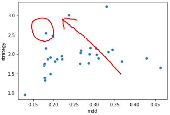
▶ 좌상단으로 갈 수록 좋은 값 : mdd는 작고, strategy 이득은 큰
sns.scatterplot(data=results, x='window_b', y='strategy', label='stragey')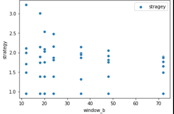
sns.scatterplot(data=results, x='window_b', y='strategy', label='stragey')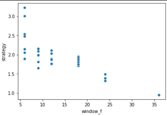
▶ window_b, window_f가 작을수록 strategy 이득이 큰편
results = pd.DataFrame(columns = ['window_b', 'window_f','strategy', 'mdd'])

window_b = np.arange(12,30,1)
window_f = np.arange(4,12,1)
i=0
for b in window_b:
    for f in window_f:
        strategy, mdd = 볼린저밴드_추세추종_찾기(window_b = b, window_f = f)
        results.loc[i, 'window_b'] = b
        results.loc[i, 'window_f'] = f
        results.loc[i,'strategy'] = strategy
        results.loc[i, 'mdd'] = mdd
        i+=1
sns.scatterplot(data=results, x='mdd', y='strategy')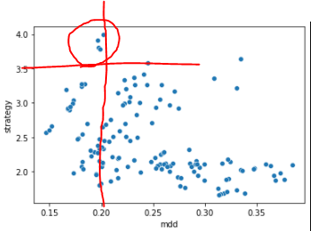
cond = results.mdd<0.2
results[cond].sort_values(by='strategy', ascending=False)[:5]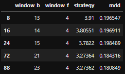
(결론) 볼린저밴드- 추세추종 기법을 활용할 경우, 최적의 하이퍼 파라미터는
window_b : 13
window_f : 4
buy_pb : 0.8
buy_mfi : 80
sell_pb : 0.2
sell_mfi : 20
그러나, 수수료 및 슬리피지를 고려하지 않은 상태다.
5000시간 ( 약 7개월 간 391% 수익률은 수수료를 고려하지 않은 상태다 )
추가)
""" 시간대별 데이터 불러오기 """
import pandas as pd
import numpy as np
import matplotlib.pyplot as plt
import pyupbit

df = pyupbit.get_ohlcv("KRW-BTC", interval = "minute60", count=10000)
data = df.copy()
print(df)
볼린저밴드_추세추종(data=data, window_b = 13, window_f=4, buy_pb = 0.8, buy_mfi = 80, sell_pb = 0.2, sell_mfi=20, chart=True)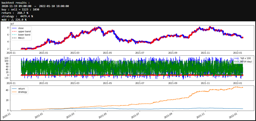
▶ 최근 7개월이 아닌 최근 14개월로 확장할 경우, 45배로 뛴다.
최근 14개월 간은 괜찮은 효과를 보여주는 알고리즘 이었던 것 같다.
■ 실전 테스트를 위해 5분봉 실험
5분봉 6개월치 데이터 백테스트
df = pyupbit.get_ohlcv("KRW-BTC", interval = "minute5", count=12*24*7*6)
data = df.copy()

볼린저밴드_추세추종(data=data, window_b = 6, window_f=3, buy_pb = 0.8, buy_mfi = 80, sell_pb = 0.2, sell_mfi=20, chart=True)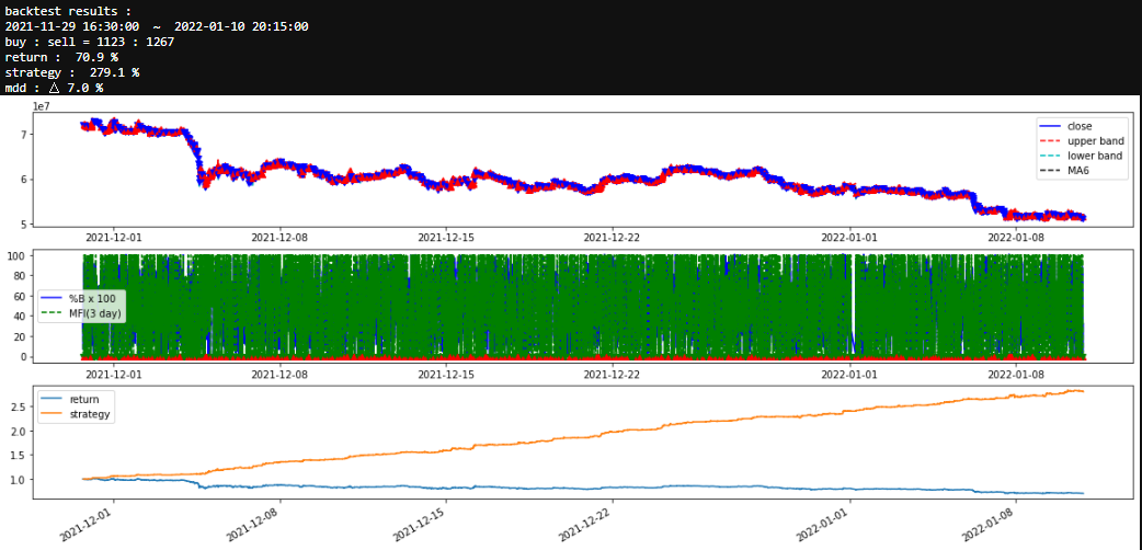
results = pd.DataFrame(columns = ['window_b', 'window_f','strategy', 'mdd'])

window_b = np.arange(5,20,1)
window_f = np.arange(3,10,1)
i=0
for b in window_b:
    for f in window_f:
        strategy, mdd = 볼린저밴드_추세추종_찾기(data=data, window_b = b, window_f = f)
        results.loc[i, 'window_b'] = b
        results.loc[i, 'window_f'] = f
        results.loc[i,'strategy'] = strategy
        results.loc[i, 'mdd'] = mdd
        i+=1
sns.scatterplot(data=results, x='mdd', y='strategy')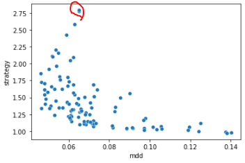
window_b=6, window_f=3 으로 실전 테스트
'STOCK > 비트코인' 카테고리의 다른 글
| 볼린저밴드-추세추종-return 계산하기(백테스트 문제점) (0) | 2022.01.11 |
|---|---|
| 볼린저밴드-추세추종 (실전 테스트) (0) | 2022.01.11 |
| 백테스트 - MLP 일봉 4년데이터 (0) | 2022.01.03 |
| 백테스트 - SMA 1시간봉 (0) | 2022.01.03 |
| 백테스트 - MLP 5분봉 volume 변수추가 (0) | 2022.01.03 |
'STOCK/비트코인' Related Articles
more


Comments