STOCK/비트코인
Time Series Forecasing - one variable
BOTTLE6
2022. 2. 9. 22:35
2달 일봉데이터를 불러와서
TimeSeries 모델에 넣어서 돌려보기
1. Library & Data load
""" 시간대별 데이터 불러오기 """
import pandas as pd
import numpy as np
import matplotlib.pyplot as plt
import pyupbit
from sklearn.metrics import mean_squared_error
from math import sqrt

data = pyupbit.get_ohlcv("KRW-BTC", interval = "day", count=60)
2. Train Test Split
dataset = data[['close']]
train_size=0.92
total_data = dataset.shape[0]
split = int((total_data * train_size))
train = dataset[0:split]
test = dataset[split:]
plt.figure(figsize=(12,6))
plt.plot(train.index, train.close, label='Train')
plt.plot(test.index, test.close, label='Test')
#plt.xticks(dataset.index, dataset.index, rotation='vertical')
plt.legend(loc='best')
plt.title("Train Test Split")
plt.show()
3. MinMaxSclaing
from sklearn.preprocessing import MinMaxScaler
mm = MinMaxScaler()
mm.fit(train)
train = pd.DataFrame(mm.transform(train), columns=train.columns, index=list(train.index.values))
test = pd.DataFrame(mm.transform(test), columns=test.columns, index=list(test.index.values))
plt.figure(figsize=(12,6))
plt.plot(train.index, train.close, label='Train')
plt.plot(test.index, test.close, label='Test')
#plt.xticks(dataset.index, dataset.index, rotation='vertical')
plt.legend(loc='best')
plt.title("Train Test Split")
plt.show()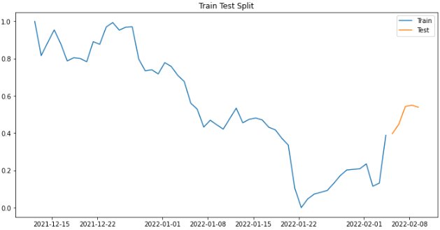
4. Modeling
def plot_figure(title, pred, train_index=train.index, test_index=test.index, y_train=train.close, y_test=test.close):
    rmse = sqrt(mean_squared_error(y_test, pred))
    print(f"{title} Mean Square Error (RMSE): %.3f" % rmse)
    plt.figure(figsize=(10,6))
    plt.plot(train_index, y_train, label='Train')
    plt.plot(test_index, y_test, label='Test')
    plt.plot(test_index, pred, label='Prediction')
    #plt.xticks(dataset["Month"], dataset["Month"], rotation='vertical')
    plt.legend(loc='best')
    plt.title(f"Predictions by {title}, RMSE : %.3f " %rmse)
    plt.show()
① Naive Approach
predictions_nv = test.copy()
# Copy the last observed Sales from training data
predictions_nv["Predictions"] = train.tail(1).iloc[0]["close"]
print (predictions_nv)
plot_figure(title = "Naive", pred=predictions_nv["Predictions"])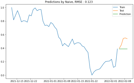
② AR (Auto Regressive)
from statsmodels.tsa.ar_model import AutoReg
model_ag = AutoReg(endog = train["close"], \
                   lags = 7, \
                   trend='c', \
                   seasonal = False, \
                   exog = None, \
                   hold_back = None, \
                   period = None, \
                   missing = 'none')
# endog: dependent variable, response variable or y (endogenous)
# exog: independent variable, explanatory variable or x (exogenous)
# lags: the no. of lags to include in the model
#       [1, 4] will only include lags 1 and 4
#       while lags=4 will include lags 1, 2, 3, and 4
# trend: trend to include in the model
#        {‘n’, ‘c’, ‘t’, ‘ct’}
#        ‘n’ - No trend.
#        ‘c’ - Constant only.
#        ‘t’ - Time trend only.
#        ‘ct’ - Constant and time trend.
# seasonal: whether to include seasonal dummies in the model
fit_ag = model_ag.fit()
print("Coefficients:\n%s" % fit_ag.params)
predictions = fit_ag.predict(start=len(train), \
end=len(train)+len(test)-1, \
dynamic=False)
predictions = pd.DataFrame(predictions, columns=['Predictions'])
predictions.index = test.index
result = pd.concat([test, predictions], axis=1)#.reindex(test.index)
plot_figure(title = "AR", pred=predictions['Predictions'])Coefficients:
intercept 0.012255
close.L1 1.198519
close.L2 -0.373919
close.L3 0.342944
close.L4 -0.348521
close.L5 0.083912
close.L6 0.019845
close.L7 0.037190
③ MA(Moving Average)
from statsmodels.tsa.arima.model import ARIMA
model_ma = ARIMA(endog = train["close"], \
                   order=(0, 0, 2))
# q = 2
# endog: dependent variable, response variable or y (endogenous)
# order: order of the model for the autoregressive,
#        differences & moving average components.
fit_ma = model_ma.fit()
print("Coefficients:\n%s" % fit_ma.params)
Coefficients:
const 0.555103
ma.L1 1.484815
ma.L2 0.821303
sigma2 0.013827predictions_ma = fit_ma.predict(start = len(train), \
end = len(train)+len(test)-1, \
dynamic = False)
plot_figure(title = "MA", pred=predictions_ma)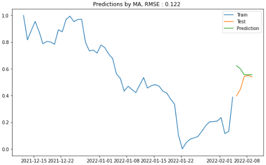
④ ARMA(Auto Regressive Moving Average)
from statsmodels.tsa.arima.model import ARIMA
model_arma = ARIMA(endog = train["close"], \
                   order = (2, 0, 1))
# endog: dependent variable, response variable or y (endogenous)
# order: order of the model for the autoregressive,
#        differences & moving average components.
fit_arma = model_arma.fit()
print("Coefficients:\n%s" % fit_arma.params)
Coefficients:
const 0.545970
ar.L1 0.170420
ar.L2 0.757241
ma.L1 0.855902
sigma2 0.005592
dtype: float64predictions_arma = fit_arma.predict(start = len(train), \
end = len(train)+len(test)-1, \
dynamic = False)
plot_figure(title = "ARMA", pred=predictions_arma)
⑤ ARIMA(Auto Regressive Integrated Moving Average)
from statsmodels.tsa.arima.model import ARIMA
model_arima = ARIMA(endog = train["close"], \
                   order = (1, 1, 1))
# endog: dependent variable, response variable or y (endogenous)
# order: order of the model for the autoregressive,
#        differences & moving average components.
fit_arima = model_arima.fit()
print("Coefficients:\n%s" % fit_arima.params)
Coefficients:
ar.L1 -0.378863
ma.L1 0.638885
sigma2 0.005580predictions_arima = fit_arima.predict(start = len(train), \
end = len(train)+len(test)-1, \
dynamic = False)
plot_figure(title = "ARIMA", pred=predictions_arima)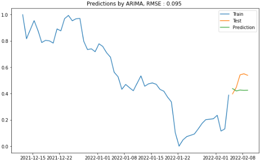
⑥ SARIMA(Seasonal AutoRegressive Integrated Moving Average)
from statsmodels.tsa.statespace.sarimax import SARIMAX
model_sarima = SARIMAX(endog = train["close"], \
                        order = (1, 1, 1), \
                        seasonal_order=(0, 0, 0, 0))
# endog: dependent variable, response variable or y (endogenous)
# order: order of the model for the autoregressive,
#        differences & moving average components.
# seasonal_order: (P,D,Q,s) order of the seasonal component of
#     the model for the AR parameters, differences,
#     MA parameters, and periodicity. s is the periodicity
#     (number of periods in season), often it is 4 for
#     quarterly data or 12 for monthly data (default, no
#     seasonal effect).
fit_sarima = model_sarima.fit()
print("Coefficients:\n%s" % fit_sarima.params)
Coefficients:
ar.L1 -0.378863
ma.L1 0.638885
sigma2 0.005580predictions_sarima = fit_sarima.predict(start = len(train), \
end = len(train)+len(test)-1, \
dynamic = False)
plot_figure(title = "SARIMA", pred=predictions_sarima)
⑦Auto ARIMA
from pmdarima.arima import auto_arima
model_aarima = auto_arima (y = train["close"], \
                           seasonal=False, \
                           stepwise=True)
# seasonal : default=True, whether to fit
#            a seasonal ARIMA.
# stepwise : default=True, the auto_arima
#            function has two modes: stepwise
#            & parallelized (slower)
ARIMA(order=(0, 1, 0)predictions_aarima = model_aarima.predict(n_periods=test.shape[0], \
X=None, \
return_conf_int=False, \
alpha=0.05)
plot_figure(title = "Auto ARIMA", pred=predictions_aarima)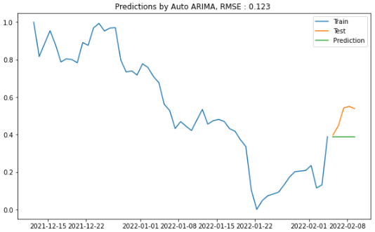
⑧ XGBOOST
dataXGB = dataset.copy()
# Restructure the data
dataXGB["Target"] = dataXGB.close.shift(-1)
# Drop the last null column because of shifting
dataXGB.dropna(inplace=True)
# Extract features & labels
X = dataXGB.loc[:,"close"].values
y = dataXGB.loc[:, "Target"].values
from sklearn.model_selection import train_test_split
X_train, X_test, y_train, y_test = \
      train_test_split(X, y, train_size = train_size, \
                       random_state = 0, shuffle=False)
import xgboost
reg = xgboost.XGBRegressor(objective='reg:squarederror', \
                           n_estimators=100)
reg.fit(X_train, y_train)
predictions_xgb = reg.predict(X_test)
predictions_xgb = pd.DataFrame({'Predictions': \
predictions_xgb})
result_xgb = pd.concat( \
[dataXGB.tail(len(X_test)) \
.reset_index(drop=True), \
predictions_xgb], axis=1)
print (result_xgb)### 오류;;;
⑨ TBATS
from tbats import TBATS
# /databricks/python/bin/pip install tbats==1.1.0
model_tbats = TBATS(seasonal_periods=(12, 28),\
              use_arma_errors=False,\
              use_box_cox=False,\
              n_jobs=None,\
              use_trend=None,\
              use_damped_trend=None)\
          .fit(train.close)
predictions_tbats = model_tbats.forecast(steps=test.shape[0])
predictions_tbatsDF = pd.DataFrame()
predictions_tbatsDF["Predictions"] = predictions_tbats.tolist()
result_tbats = pd.concat([test.reset_index(drop=True), \
                           predictions_tbatsDF], axis=1)
print (result_tbats)
plot_figure(title = "TBATS", pred=predictions_tbatsDF["Predictions"])
⑩ ETS
from statsmodels.tsa.holtwinters import ExponentialSmoothing
model_es = ExponentialSmoothing(endog=train["close"], \
                                trend='add', \
                                seasonal='add', \
                                seasonal_periods=12, \
                                damped=True)
# Parameters
# endog : The time series to model.
# trend : Type of trend component (optional);
#         options: "add", "mul", "additive",
#                  "multiplicative", None
# seasonal : Type of seasonal component (optional);
#         options: "add", "mul", "additive",
#                  "multiplicative", None
# damped_trend : Should the trend component
#                be damped (optional)
fit_es = model_es.fit(optimized=True, \
use_boxcox=False, \
remove_bias=False)
predictions_es = fit_es.predict(start=test.index[0], \
end=test.index[-1])
predictions_es
plot_figure(title = "ETS", pred=predictions_es)
5. 예측력이 가장 좋은 모델이었던 TBATS로 예측해보기
steps = 5
history = mm.transform(dataset)
model_tbats = TBATS(seasonal_periods=(12, 28),\
              use_arma_errors=False,\
              use_box_cox=False,\
              n_jobs=None,\
              use_trend=None,\
              use_damped_trend=None)\
          .fit(history)
predictions_tbats = model_tbats.forecast(steps=steps)
predictions_tbatsDF = pd.DataFrame()
predictions_tbatsDF["Predictions"] = predictions_tbats.tolist()
predictions_tbatsDF["Predictions"]
0 0.542856
1 0.485745
2 0.498366
3 0.505518
4 0.377700steps=5
delta = dataset.index[-1]-dataset.index[-2]
new_index = [ dataset.index[-1]+ delta*(i+1) for i in np.arange(steps)]
plot_figure(title = f"TBATS {steps}days", pred=predictions_tbatsDF["Predictions"], \
train_index = dataset.index, test_index=new_index, \
y_train=history, y_test=np.zeros(steps))
향후 5일간 하락할 것으로 예상
steps = 15
predictions_tbats = model_tbats.forecast(steps=steps)
predictions_tbatsDF = pd.DataFrame()
predictions_tbatsDF["Predictions"] = predictions_tbats.tolist()
predictions_tbatsDF["Predictions"]

delta = dataset.index[-1]-dataset.index[-2]
new_index = [ dataset.index[-1]+ delta*(i+1) for i in np.arange(steps)]

plot_figure(title = f"TBATS {steps}days", pred=predictions_tbatsDF["Predictions"], train_index = dataset.index, test_index=new_index, y_train=history, y_test=np.zeros(steps))
steps = 30
predictions_tbats = model_tbats.forecast(steps=steps)
predictions_tbatsDF = pd.DataFrame()
predictions_tbatsDF["Predictions"] = predictions_tbats.tolist()
predictions_tbatsDF["Predictions"]

delta = dataset.index[-1]-dataset.index[-2]
new_index = [ dataset.index[-1]+ delta*(i+1) for i in np.arange(steps)]

plot_figure(title = f"TBATS {steps}days", pred=predictions_tbatsDF["Predictions"], train_index = dataset.index, test_index=new_index, y_train=history, y_test=np.zeros(steps))
6. 데이터를 2달에서 3달로 변경
data = pyupbit.get_ohlcv("KRW-BTC", interval = "day", count=90)
dataset = data[['close']].copy()
mm = MinMaxScaler()
mm.fit(train)
dataset = pd.DataFrame(mm.transform(dataset), columns=dataset.columns, index=list(dataset.index.values))
plt.figure(figsize=(12,6))
plt.plot(dataset.index, dataset.close, label='Train')
#plt.xticks(dataset.index, dataset.index, rotation='vertical')
plt.legend(loc='best')
plt.title("Train Test Split")
plt.show()
# 학습
history = dataset.copy()
model_tbats = TBATS(seasonal_periods=(12, 28),\
use_arma_errors=False,\
use_box_cox=False,\
n_jobs=None,\
use_trend=None,\
use_damped_trend=None)\
.fit(history)
steps = 5
predictions_tbats = model_tbats.forecast(steps=steps)
predictions_tbatsDF = pd.DataFrame()
predictions_tbatsDF["Predictions"] = predictions_tbats.tolist()
predictions_tbatsDF["Predictions"]

delta = dataset.index[-1]-dataset.index[-2]
new_index = [ dataset.index[-1]+ delta*(i+1) for i in np.arange(steps)]

plot_figure(title = f"TBATS {steps}days", pred=predictions_tbatsDF["Predictions"], train_index = dataset.index, test_index=new_index, y_train=history, y_test=np.zeros(steps))
steps = 15
predictions_tbats = model_tbats.forecast(steps=steps)
predictions_tbatsDF = pd.DataFrame()
predictions_tbatsDF["Predictions"] = predictions_tbats.tolist()
predictions_tbatsDF["Predictions"]
delta = dataset.index[-1]-dataset.index[-2]
new_index = [ dataset.index[-1]+ delta*(i+1) for i in np.arange(steps)]
plot_figure(title = f"TBATS {steps}days", pred=predictions_tbatsDF["Predictions"], train_index = dataset.index, test_index=new_index, y_train=history, y_test=np.zeros(steps))
steps = 30
predictions_tbats = model_tbats.forecast(steps=steps)
predictions_tbatsDF = pd.DataFrame()
predictions_tbatsDF["Predictions"] = predictions_tbats.tolist()
predictions_tbatsDF["Predictions"]

delta = dataset.index[-1]-dataset.index[-2]
new_index = [ dataset.index[-1]+ delta*(i+1) for i in np.arange(steps)]

plot_figure(title = f"TBATS {steps}days", pred=predictions_tbatsDF["Predictions"], train_index = dataset.index, test_index=new_index, y_train=history, y_test=np.zeros(steps))
7. 데이터를 2주일로 변경
(참고) https://cprosenjit.medium.com/10-time-series-forecasting-methods-we-should-know-291037d2e285
향후 계획
- 다변량 알고리즘 활용, 딥러닝 활용
- 여러 시계열 모델, 머신러닝 모델 결합해보기